Stroop task in OpenSesame

Note: The text below is adapted from the OpenSesame guide by James E. Bartlett licensed under CC-By Attribution 4.0 International.

Tutorial 1. Stroop Task

Creating the Stroop task

To get a look at OpenSesame, we will first create one of the simplest and most famous psychology experiments, the Stroop task. This demonstrates the automaticity of reading as identifying the font colour of a congruent word (e.g. blue) is faster than identifying the font colour of an incongruent word (e.g. blue). When the word and colour are incongruent, the interference causes a delay in identifying the colour of the font. We will create a single block of trials to demonstrate the task. As you go through the guide, I recommend saving your experiment every time you reach a new sub-heading like the next line.

Creating a new experiment

If you open OpenSesame on your computer, you should get a window that looks like this:

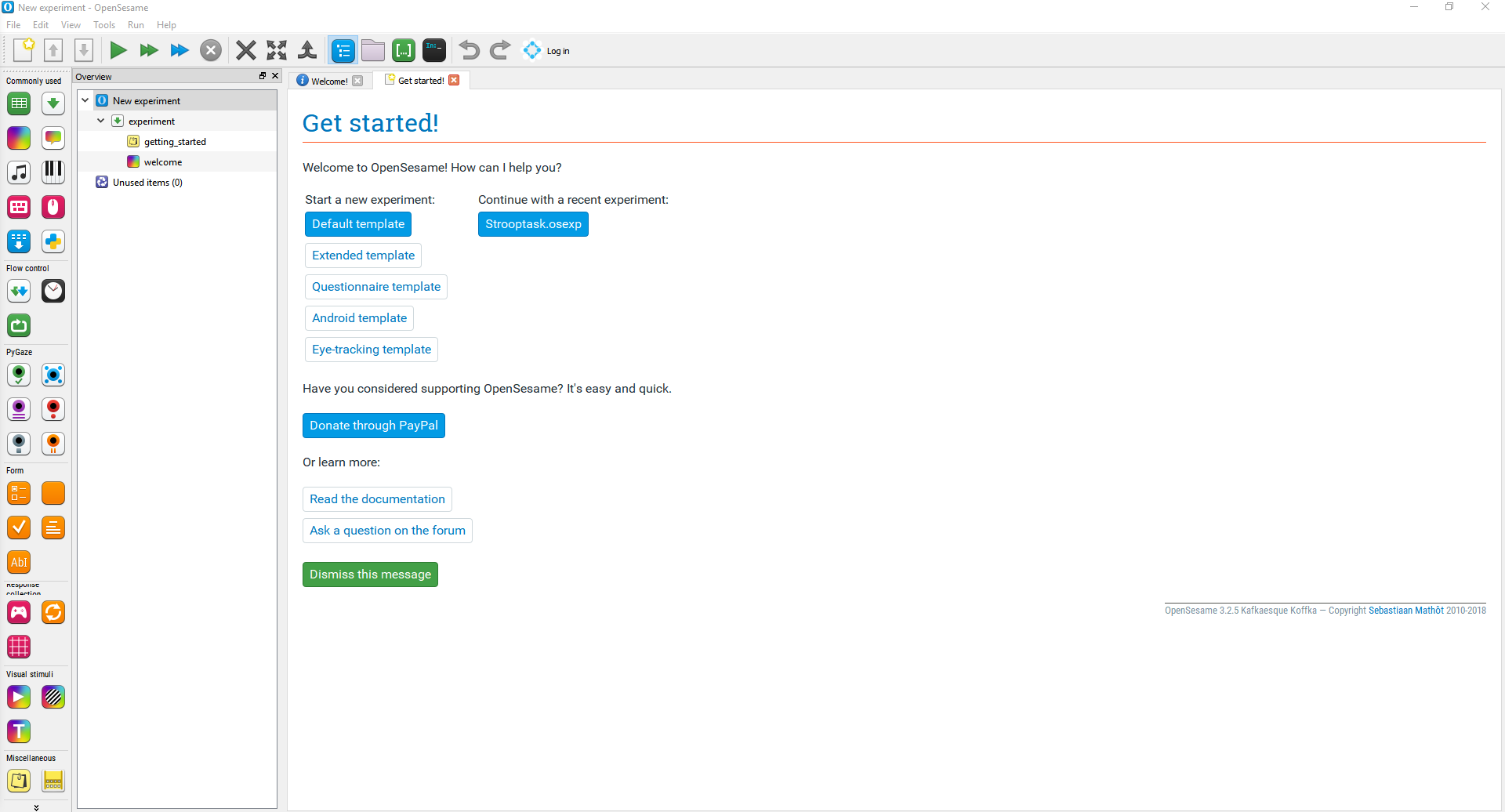
To help you start an experiment, there are some templates that you can use. We are going to use the default template as we are going to make a single block of trials from scratch to demonstrate the building blocks of OpenSesame. Once you click on this, a new screen will appear and you will be able to change any of the general properties of the task. It is a good idea to give your experiment an informative name. You can do this by clicking where it says New experiment in blue, and editing the text. Press the return key to save the new name. Make sure you change the resolution to your monitor’s dimensions. If you are not sure what the resolution of your monitor is, you can look in the display settings of your computer. Once you have changed these, the general properties window should look like this:

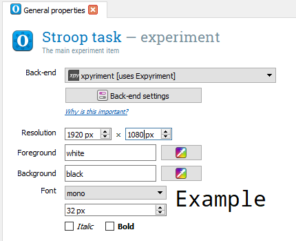
There are a few settings to explain here. Foreground and background refers to the colour of the screen and the elements displayed on it. We will keep the background black so the participant does not have to look at a dazzling white screen, and the foreground white to make it easy to read on a black background. I would also recommend increasing the default size of the font to 32, as 18 is too small to read and it saves you changing it every time you create a new component.

The building blocks of creating an experiment

Before making the Stroop task, we will go over some of the basics of structuring an experiment in OpenSesame. The design of your experiment will be shown in the Overview window, and it is displayed sequentially down the screen from the components at the start of the experiment to the components at the end of the experiment. The backbone of an experiment is created through loop and sequence components. A loop component repeats what is inside it and defines any variables to use. 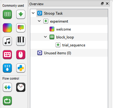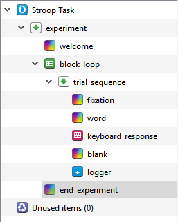A sequence component contains other components such as a screen showing text that make up a single trial. Therefore, you would place a sequence component within a loop component to control how many times the sequence is repeated. Drag a loop component and place it after welcome in the overview window, and drag a sequence component and place it inside the loop. When you release the sequence, it will ask whether you want it placing into the loop or after the loop. Press into the loop and make sure they are both given informative names such as block_loop for the loop component and trial_sequence for the sequence component. For the names of components, there are a number of rules you need to follow. They cannot start with numbers, and you cannot include any spaces. If you need spaces to make it easier to read, use an underscore. You should now have a window that looks like this: Therefore, once we define our variables later, trial_sequence and everything in it will repeat for however many times you specify in block_loop. We will now create a single trial within trial_sequence. In most psychology experiments, you include a fixation cross to start a trial and focus the participant’s attention in the location where you will be presenting the stimulus.

Creating the fixation dot

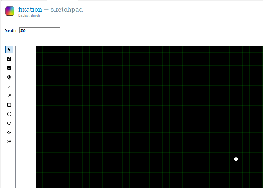
This can be created using a sketchpad component . This is a very flexible component where you can present text, shapes, and images. The sketchpad window has a list of elements on the left hand side and a black screen with green lines to show where on the screen the elements would be placed. OpenSesame has a very handy fixation cross element called fixdot . Click on the fixdot element and this will turn your mouse into a pen icon. If you move the mouse around the black gridded screen, the coordinates are shown in the top right corner, and will change as you move around the screen. Place the fixdot element at 0,0 in the middle of the screen where the two green lines meet. This will place the fixdot in that position. There are two more things to change. Firstly, we can modify how long the stimuli are presented for by changing Duration. The default is keypress which would mean the screen will not disappear until the participant presses a button. We can change this to 500 to make the screen disappear after 500ms. Whenever you specify a duration in OpenSesame, it is stated in milliseconds. Therefore, to present something for 1 second, we would need to write 1000. Finally, we can change the name of the component to something informative such as fixation. You should now have a screen that looks like this:

Creating the word component

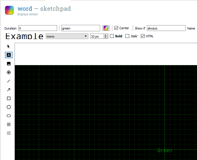
In the Stroop task, participants are shown colour words and the font is either the same colour as the word (congruent) or a different colour to the word (incongruent). Therefore, the next thing we need to do is create another sketchpad component to present the words. Drag a sketchpad component and place it after fixation in the trial sequence. Name it word to keep track of all the components. This time instead of inserting a fixation cross, we need a text element . After you have selected the text element, change the colour to green (all lowercase, it will say white by default). This will turn your mouse into a pen, and you need to click in the middle of the screen at 0,0 again to place it. When you click, it will ask you to enter some text. For now, just enter ‘Green’ as we want to show the participants colour words. This time, change Duration to 0. This does not mean that we never want it appearing on the screen, but we want it to only remain on the screen until a participant makes a response, which will require the next component keyboard_response. For the word component, you should have a window that looks like this:

Creating the keyboard response component

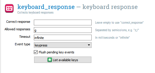
The next component is keyboard_response . Drag this from the menu and place it after word. We need this to tell OpenSesame which keyboard responses are allowed and which responses are correct. For now, we only have one green word, so the only response we need is ‘g’. If you are ever unsure of what the valid name of the key you need is, click on List available keys. We will not specify a correct response yet. We can leave Timeout to infinite, so the word will remain on the screen until the participant presses ‘g’ on the keyboard. As we set the duration of the word component to 0, the amount of time it is presented for is determined by keyboard_response. A keyboard response component does not display on the screen, so it keeps the display from the previous sketchpad component. A common mistake is to set a time for both components. This would not allow you to record any response until the Duration of the word component has ended. This could really confuse participants as they would have to respond twice for the trial to end. You should now have a screen that looks like this for keyboard_response:

Creating a blank screen

After the keyboard response, we will place another sketchpad component to signal the end of the trial. This time it will just be a blank screen presented for 200ms. You can do this yourself based on the previous sketchpad components and name it blank. We do not need to add any text or fixdot elements.

Creating the logger component

The next component that we need is a logger to save the data. OpenSesame does not save the responses by default, so you need to create a logger to save the data from each trial. Drag a logger component and place it after blank. For most experiments, you can just keep the default option here. It just saves every available variable on each trial.

Creating the end of experiment screen

The final component we need is a screen to tell the participant the experiment has finished. Without this, the experiment just closes which can make the participant panic and think they have done something wrong. Create a new sketchpad component called end_experiment and place it after block_loop. Make sure it is not in trial_sequence. If you drop it on block_loop, you can select insert after block_loop. Here we just need a brief message saying ‘The experiment has now finished. Press any key to exit’. In order to create this, select a text element , click in the middle of the screen, and enter the message. Now the participant is fully aware that the experiment has finished successfully. Make sure Duration is set to keypress. You should now have an experiment that looks like this in the Overview window:

Modifying the welcome message

The final thing to do before we test whether the experiment works is to change welcome. By default, this lists the version of OpenSesame that you are using. You can edit the pre-existing text by hovering over the text until it turns a light grey colour, and double-clicking. Change the text to something like ‘Welcome to the experiment, press any key to begin.’. We will make this more informative later on, but for now, this will do. All that matters is this sketchpad component has a keypress duration, as we want the participant to start the experiment when they are ready.

Time to test the experiment

Now it is time to make sure everything works! In the menu, there are three arrow buttons. If you were collecting data from a participant, you would press the big green triangle to run the experiment full screen. The two green triangles runs the experiment in a separate window. The two blue triangles allow you to quickly run the experiment in a separate screen to make sure everything is working. It is usually a good idea to test your experiment using quick run, as if your experiment crashes, you can force it to quit. If you click quick run, your experiment should successfully run in a small window. If it does not run, look back at all of the instructions and make sure you have not made any typos, and all the components are where they should be. Remember to press ‘g’ to indicate the color is green. We only have one trial up to yet, so it will only last around one second. However, it is helpful to keep testing an experiment to make sure it works before you add something else. It makes it much easier to debug your experiment if you know it worked previously. This means you only need to investigate the changes you have made since it last worked. Your sanity will thank you if you make incremental changes, saving and running the experiment after every addition. Now that we know one trial works, we can add in multiple words and make the colour of the word change.

Manipulating the presentation of word and colour

When we created the word component, we specified green as the word and colour. For the Stroop task, we want different words and colours depending on the condition. Therefore, we need to make both the word and colour variable for each trial. We need to do this in two steps. Firstly, we need to specify our conditions in block_loop (remember this is where we define our variables and control how many times sequence runs). We then need to change word to allow the word and colour to change every trial. We will start with block_loop.

Editing the block_loop component

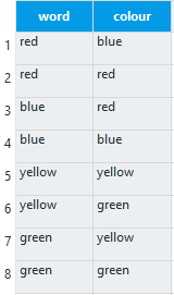
If you click on block_loop, it looks like an Excel sheet with lots of cells. This is where we can define our variables and conditions. The rules here are every column is a variable, and each row is an individual condition. The variables must have unique names, so you cannot repeat a variable name in the same or a different loop component. The first column will be called ‘empty_column’ by default. We will change this to ‘word’. We will change the second column to ‘colour’. It makes it easier if you use lower case letters as the variable names are case sensitive. We then need to populate the cells. We will have four words and colours: red, blue, yellow, and green. We want there to be some congruent and incongruent trials, so write each colour twice in the word column. In the colour column, we will pair red with blue, and yellow with green. So for each word, you should have one congruent colour and one incongruent colour. The grid should look like this:

We also need some additional variables that will be helpful for analysing the data later. We need a column called ‘congruent’ and a column called ‘correct_resp’. In the congruent column, write a 1 for every time the word and colour match, and a 0 for every time they do not match. In programming, 1 usually means true and 0 usually means false. This means that when we get the data afterwards, we can sort the responses by congruency and calculate whether the reaction times are longer in the incongruent condition. We also need to specify what is the correct response in order to use it in keyboard_response. In the correct_resp column, write the first letter of the colour variable for that row, e.g. r for red. You should now have a full grid like this:

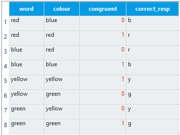
This will create 8 trials, one for each row. Remember how it is the loop components that determine how many times the sequence component repeats. In other words, for every loop around trial_sequence, it will use one of these rows. Our next task is to edit the word component to use these new variables.

Editing the word component

If you click on the word component, Green is still in the middle of the screen with green font. We need to click on the settings icon in the top right corner and click on view script. We need to change two things here: the color and text arguments. At the moment, these are static and just present Green every time the component is called. OpenSesame lets you specify arguments using variables defined in a loop by entering the variable name surrounded by square brackets. For color, you should change it to say color = [colour]. This means that every time the component is called, the colour of the word will be determined by the colour variable in block_loop. We can then do the same for word and make sure it says text = [word]. Be very careful with your typing here as the variables are case sensitive. It should be typed exactly as it is in block_loop. One of the biggest causes of experiments not working is typos. You need an eagle eye to spot where you have made a mistake. The script should now look like this:

Click on apply and close in the top right corner and we can move on to keyboard_response.

Editing keyboard_response

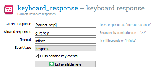
We can now specify what variable determines a Correct response and enter several Allowed responses. In block_loop, we created a variable called correct_resp to tell OpenSesame what response should be provided. We need to use the same trick as in the script for word and enter ‘[correct_resp]’ to tell OpenSesame it should look for a variable. We then need to specify the four different responses that are allowed (g; r; b; y) in the Allowed responses box. It is important that the letters are separated by a semicolon and not a comma. After this, you should have a window that looks like this:

Test the experiment

We can now test it works again using quick run. It should run for 8 trials providing you have followed all the instructions closely. If you get an error message, use the instructions to try and locate the problem. It will probably be a stray typo in one of the variable names you have entered, so make sure it is all typed out exactly as in the instructions.

Increase the number of trials

Now that we know everything works fine, we can scale the experiment up to provide more trials. If we go back to block_loop, we can change the Repeat value to 4. This repeats all of our conditions 4 times to produce 32 trials. You will find that cognitive tasks repeat stimuli many times and take the average. We could specify all 32 trials in the block_loop grid, but doing it like this is much more efficient. One of the important settings to highlight now is Order. The default is random, which mixes our 8 rows up every time we run the experiment. This is usually the setting you will use as randomising the order helps to avoid presentation order being a confounding variable. The alternative is sequential. This calls the conditions in the exact order that you wrote them in. This can occasionally be useful if the order of presentation is important.

Run the experiment full screen

Now it is time to run the experiment in full screen (the single green arrow) and enter a subject number. In other places, this could be called a participant number or code, but they mean the same thing. It is just the method you are using to label each participant. When you run an experiment, you will need to label all of your participants. OpenSesame asks you to provide a number, and then asks you to specify where you want to save the file. Make sure you create an easily identifiable folder to store your data. When it comes to saving the file, it is better to name your file clearly with a three digit participant number, e.g. stroop-001. This makes it easier to find and organise the file later, and creating a three digit code helps with ordering the files. Click save and run all 32 trials. We will now take a look at the data to see how we could analyse it.

Analysing response time data from the Stroop task

Every time you run the experiment, OpenSesame saves the data as a .csv file. This stands for comma-separated values. If you have Microsoft Excel or Openoffice on your computer, you should be able to double click on the file and open it. As we told the logger we want every variable saving, we get many columns. The file should have 32 rows of data and look similar to this:

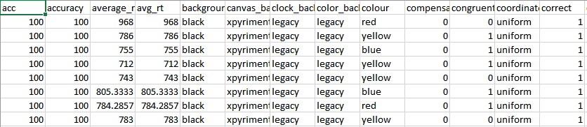
We do not need every value here, but it is safer to save everything and use what we need. The key variables for analysing the data in this experiment are congruent, correct, and response_time. We can use SPSS to import and process the data for us and see whether we can see the Stroop effect in 32 trials. There are two versions to the import instructions depending on whether you are using version 23 or 25 of SPSS.

Importing the data in SPSS version 23

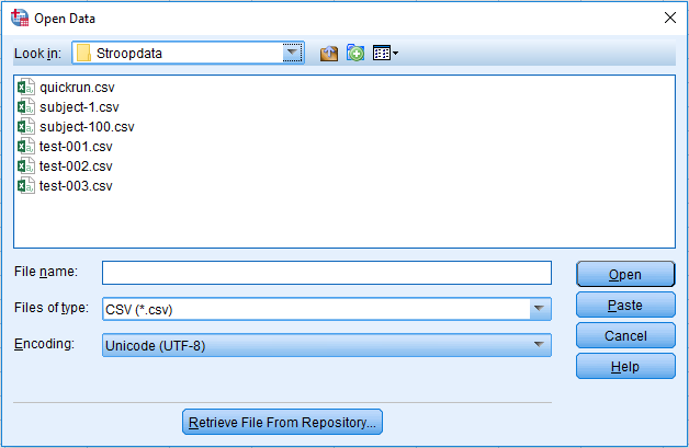
Open SPSS and select open new dataset. This will present you with a blank data view screen to work from. In the main menu, click File > Open > Data. This will present you with a box to Open Data in. In order to open the data file, you will need to change Files of type to CSV (*.csv). If you do not change this, SPSS will just look for SPSS .sav data files. At the top of the box there is a drop-down menu called Look in. This is where you need to search to find where you saved the data on your computer. The window should look like this:

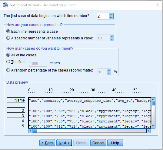
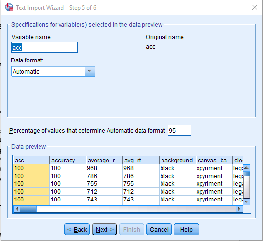
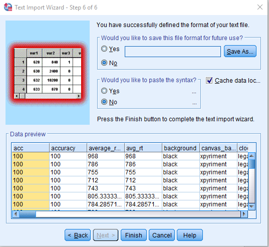
Select the file you need, and click Open. This will open the Text Import Wizard which requires six steps. 1) We do not have a predefined format, so it should say no by default. Click Next. 2) How the variables are arranged should be set to Delimited, the variable names are included at the top of the file, so it should be set to yes, and the decimal symbol should be set to Period. Some international formats use a comma for the decimal symbol, so if you have data in an international format, this would need changing to Comma. Click Next. 3) The first case begins on line number 2, each line represents a case, and we want to import All of the cases. Click Next. 4) The delimiters should be set to Comma and Space by default, and text qualifier set to Double quote. Click Next. 5) This page provides you with the option to change each variable name, but we can change these later if necessary. Click Next. 6) We do not need to save the file format for future use, and we do not need to paste the syntax. Click Finish to complete the process and the data will be available in the data view screen of SPSS. The whole process from above is shown in the following series of screenshots:

Importing the data in SPSS version 25

If you have version 25 of SPSS, you can follow the instructions for version 23 and the process works, but in version 25 there is a more streamlined option for importing data. Open SPSS and select new dataset. There is an option to import data if you click file > Import Data > CSV Data and select the experiment file from where you saved it on your computer. You should have a screen that looks similar to this:

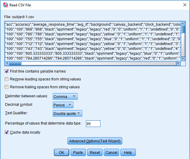
You should not have to change any of the default settings apart from if your data is saved in an international format. Some countries use a comma for a decimal symbol. If this is the case, you would need to change Decimal Symbol to comma. If not, you should just need to press OK.

Processing the data

Before we do any analysis, it is important to process the data. Conventionally, we remove any incorrect responses as they may be unreliable. In addition, we should ensure that there are no problematic outliers. In the simplest case, there are response times that can be considered too fast or too slow. Anything below 100-200ms is unlikely to be a real response to the stimulus, as there is not enough time for the participant to perceive the stimulus and make a response. Conversely, response times above 1000-2000ms can be considered too slow and the participant may have been distracted. Response times on simple tasks are usually in the range of 400-700ms. A range of values at each end of the threshold have been presented as there is no one solution. It is important to read articles similar to the study you are conducting to see what they have done and justify your own decisions.

For the next step in the outlier removal procedure, some studies will remove response times above and below certain thresholds to ensure the response times are approximately normally distributed. The most common of these is two or three standard deviations above and below the mean (Lachaud and Renaud, 2011). Despite being commonly used, there is good reason not to do this including being biased by the very outliers they are trying to remove (Leys et al., 2013). If you are interested in using a more robust outlier removal method, Leys et al. (2013) present an alternative using the absolute median deviation. As the outlier removal method differs between studies and topic, in this guide we will just focus on removing incorrect responses, and response times below 100ms and above 1000ms. When it comes to designing your own studies, you will need to look more closely at these articles and methods.

Identifying extreme responses

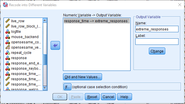
In order to process the data, we will do it in two steps. The first is to create a new variable that defines any outliers beyond 100ms and 1000ms. On the main menu, click on Transform > Recode into Different Variables. Drag response_time into the white box, and type a new Output Variable Name called something like ‘extreme_responses’ and click Change. You should now have a screen that looks like this:

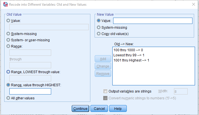
Now click on Old and New Values. This allows us to recode response_time into several values by specifying individual values, or a range of values. Our acceptable response times are 100-1000ms, so we will define three ranges for new values. 1) Click on Range and enter 100 in the first white box and 1000 in the second white box. We then need to specify a New Value for these responses. These are acceptable, so we can code them as 0. Finally click Add, and they will appear in the Old –> New box. Now we want to specify our extreme responses. 2) Click on Range, LOWEST through value and enter 99. This means we are taking the range from the lowest value in response_time to 99, as above 100ms is OK. Select a New Value of 1, and click Add. 3) Click on Range, value through HIGHEST, and specify 1001. Select a New Value of 1, and click Add. You should have a window looking like this:

Click Continue and OK, and SPSS will create a new column called extreme_responses. Any row with a 0 is fine, and any with a 1 is outside of our boundary and considered an extreme response.

Filtering out extreme and incorrect responses

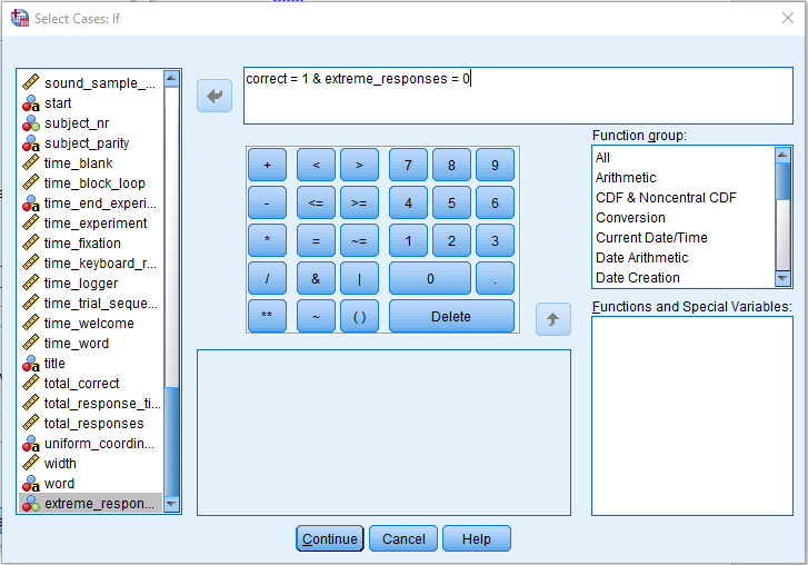
We can now get SPSS to ignore any of our incorrect and extreme responses. You can do this in SPSS by clicking on the main menu Data > Select Cases. You then need to select ‘if condition is satisfied’ and click on the ‘if’. We can drag correct into the white box, and make sure it says ‘correct = 1’. This means that we only want cases which has the value 1, indicating a correct response. We also want to exclude our extreme responses, so write ‘& extreme_responses = 0’. This means we only want to include responses within our boundary. It should now say ‘correct = 1 & extreme_responses = 0’. The window should look like this:

Click Continue and then OK, and any responses not meeting our criteria will be crossed out. For my data, there are four cases that are either incorrect or considered extreme. When we run any analyses, this will not be included but does not delete them.

Getting the outcome variable

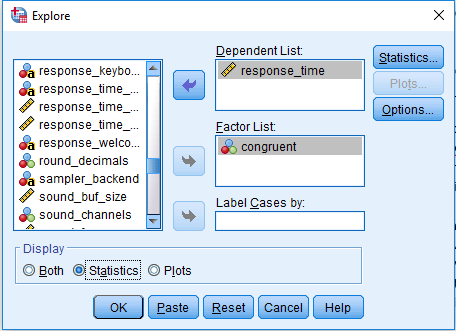
To get the average response for our two conditions, we can click on Analyze > Descriptive Statistics > Explore. Drag response_time into Dependent List and congruent into Factor List. Select Statistics under Display. The window should look like this:

Press OK to produce the output. This will provide the descriptive statistics split by the congruent variable. For the average, we will look at the median response time. Response times tend not to be normally distributed and the mean is often not an appropriate choice. Although it is not perfect, the median is a better choice than the mean in the presence of a skewed distribution with outliers (see Ratcliff, 1993 for a technical paper on dealing with response time outliers). For my data, my median response is 668ms when the colour and word are congruent, and 787ms when they are incongruent. This shows that even in 28 (excluding the four removed) trials you can see the Stroop interference effect. For a real experiment, it would be better to include many more trials as you will get a more accurate estimate, but this is fine for demonstration purposes. If this was entered in SPSS to analyse the data for each participant in an experiment, you would need the variables organised something like this:

participant	congruent_rt	incongruent_rt
1	668	787

Hopefully, you have also seen how it is good to think in advance how you will analyse the data. This last section is one of the most important tips when designing experiments. Design it with the analysis in mind. It is better to realise now that you have overlooked something than when you have already collected data from 20 participants. You will find that you are testing your experiments out several times before the participants in order to catch any mistakes in creating the experiment, and to ensure you have all the variables you need to analyse the data when you have finished.

Glossary

Argument A value, setting, or piece of information provided by the user in computer programming, normally in a function. This may also be called a parameter.

Block A collection of trials. Blocks group the trials together with a particular theme (e.g. a unique cue is presented or a different response is required in each block). Alternatively, it justs helps to organise the trials and allow the participant to have a break in between.

Boolean operator A system of algebra used to represent logical propositions, and can provide a binary response of either true or false. For example, whether two words are the same which could be true (dog == dog) or false (dog == cat).

Cue A stimulus that elicits or signals a particular behaviour. This has quite a broad definition. In one experiment, it could be a picture of a cigarette to elicit craving in a smoker, and in the next it could be a shape on a screen that requires a particular response.

Debugging The process of finding and removing errors from your experiment or script. It is an exercise in problem solving.

Fixation cross / dot A small cross or dot (e.g. +) in the centre of the screen to attract the participant’s attention at the start of a trial.

Function A section or unit of a programme that performs a specific task. You can consider it to be a procedure or routine.

Graphical User Interface (GUI) An interface that allows users to interact with the programme using icons and visual indicators. For example, being able to select options through a menu by clicking your mouse on the screen.

Integer A whole number (e.g. 1), not a decimal (e.g. 1.3).

Inter-Stimulus Interval (ISI) The amount of time between two or more separate stimuli.

Inter-Trial Interval (ITI) The amount of time between separate trials.

Loop Controls the repetition of several trials and allows things to vary on each repetition.

Python A “high-level general purpose” programming language. See https://www.python.org/ for more details.

Response The action of a participant, e.g. the time it takes to press a button (reaction/response time), when presented with a stimulus.

Script A list of commands/code that is executed by the programme, in this case Python.

Stimulus An object or event that signals a response.

Stimulus Onset Asynchrony (SOA) The amount of time between the onset of one stimulus and the onset of the next stimulus.

Syntax A set of rules that defines the combinations of symbols that are considered to be a correctly structured document in a particular programming language.

Trial Presenting one or more stimuli and recording a response. Typically trials are repeated many times to calculate the average response.

Exercises

Excercise 1. Change stimulus duration

Change the stimulus duration from infinite to 1000 ms. What happens when you fail to respond in time? In particular, check the values of the columns correct_… and response_… in the log file.

References

Brysbaert, M., & Stevens, M. (2018). Power analysis and effect size in mixed effects models: A tutorial. Journal of cognition, 1(1).

Detandt, S., Bazan, A., Schröder, E., Olyff, G., Kajosch, H., Verbanck, P., & Campanella, S. (2017). A smoking-related background helps moderate smokers to focus: An event-related potential study using a Go-NoGo task. Clinical Neurophysiology, 128(10), 1872–1885

Mathôt, S., Schreij, D., & Theeuwes, J. (2012). OpenSesame: An open-source, graphical experiment builder for the social sciences. Behavior research methods, 44(2), 314-324

Lachaud, C. M., & Renaud, O. (2011). A tutorial for analyzing human reaction times: How to filter data, manage missing values, and choose a statistical model. Applied Psycholinguistics, 32(2), 389-416.

Leys, C., Ley, C., Klein, O., Bernard, P., & Licata, L. (2013). Detecting outliers: Do not use standard deviation around the mean, use absolute deviation around the median. Journal of Experimental Social Psychology, 49(3), 764–766.

Peirce, J. and MacAskill, M. (2018). Building Experiments in PsychoPy. London: SAGE.

Petit, G., Kornreich, C., Noël, X., Verbanck, P., & Campanella, S. (2012). Alcohol-related context modulates performance of social drinkers in a visual Go/No-Go task: a preliminary assessment of event-related potentials. PloS one, 7(5), e37466

Rass, O., Fridberg, D. J., & O’Donnell, B. F. (2014). Neural correlates of performance monitoring in daily and intermittent smokers. Clinical Neurophysiology, 125(7), 1417–1426

Ratcliff, R. (1993). Methods for Dealing With Reaction Time Outliers. Psychological Bulletin, 114(3), 510–532.

Wessel, J. R. (2018). Prepotent motor activity and inhibitory control demands in different variants of the go/no-go paradigm. Psychophysiology, 55(3), 1–14