Flanker task in OpenSesame

Note: The text below is adapted from the OpenSesame guide by James E. Bartlett licensed under CC-By Attribution 4.0 International.

Tutorial 1. Eriksen Flanker task

The Stroop task you programmed last time is probably the most famous task in the whole of psychology. Without knowing the specific details, you might be able to have a go at creating a version of it yourself. However, what would you do if you came across an unfamiliar task that was described in a study you want to extend or replicate?

How do you recreate a psychology experiment?

The aim of learning how to use OpenSesame is to enable you to create psychology experiments that you can use in your research. However, what kind of experiments can you create and where do you find out how to create them? In all empirical psychology articles, there will be a method section outlining how the authors conducted their study. If this is written well enough, it should allow you to recreate their study as close as possible. In a lot of studies that use behavioural tasks, the authors provide diagrams of how their tasks are designed. The following diagram is from an EEG study by Rass et al. (2012).

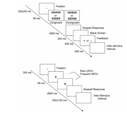
In the second part of this section, we will create the task on the top which is called the Eriksen Flanker task. This follows a similar principle to the Stroop task as it aims to measure the impact of interference on task performance. However, instead of looking at word colour, it uses distracting information. The aim of the task is to identify the middle letter in a five letter string. The four outer letters are distractors, and on some trials they are congruent, and on others they are incongruent. Studies usually find that response times are slower in the incongruent condition than the congruent condition.

What is the structure of each trial?

We will go through the diagram above step by step in order to decode how it is designed. In this experiment a trial consists of a central fixation cross which stays on the screen for a random interval between 150-250ms. This randomness is usually introduced to stop participants just mindlessly clicking buttons to predictable stimuli. A stimulus then appears on the screen for 80ms. This period is sometimes called the Stimulus Onset Asynchrony (SOA), or for how long the stimuli remain on the screen. There are two conditions for the stimuli: congruent (HHHHH or SSSSS) or incongruent (SSHSS or HHSHH). For this task, the participant has to identify the middle letter by pressing either the letter ‘s’ or ‘h’ on the keyboard. After the stimulus has disappeared, there is a blank screen where the participant has up to 800ms to provide a response. After the response, a blank screen is presented for 300ms. The participant is then provided feedback to let them know whether they pressed the correct button or not. A ‘+’ is shown for a correct response and a ‘-’ is shown for an incorrect response. Finally, an inter-trial interval (ITI; although confusingly this is called an inter-stimulus interval despite indicating the end of a trial) is shown on the screen for 500ms to indicate the end of a trial.

How is the whole experiment organised?

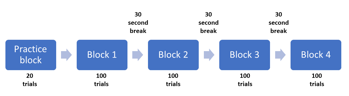
Now that we know how one trial is structured, we can see how many times this is repeated to form a block of trials. In the method section, there are more details about how many trials are included. In order for the participants to understand they are completing the task accurately, they are provided with 20 trials in a practice block. The authors then explain that participants completed four blocks each containing 100 trials for a total of 400 trials. Between each block there is a rest period for the participant, but it does not say how long this period is. We will provide participants with a short 30 second break. Finally, we know that there are an equal number of congruent and incongruent stimuli in each block. As we have two types of congruent and incongruent stimuli, we can take a good guess that each one of these is presented 25 times in each block. The authors provide us with a diagram of each trial, but we can visualise the structure of the whole experiment like this:

This is the amount of information you need from an article to enable you to recreate the task the authors used. This is a particularly good example with the only missing information being the duration of the breaks, a relatively minor detail. You should be prepared to come across substantially less helpful authors that do not provide sufficient details. This is usually the case when it comes to tasks that use images. These are not normally shared or even described. Hopefully this will also demonstrate the importance of fully describing your experiment in a report or dissertation. Try and imagine you are the other researcher trying to recreate the task from your instructions. Now that we know how the task is designed, the next step is to recreate it in OpenSesame.

Creating the Eriksen Flanker Task in OpenSesame

For this experiment, we will use the extended template rather than the default. This provides a helpful starting point by creating the basic outline of an experiment. This includes: instructions, a practice block, an experimental block, and an end of experiment message. The template should look like this when you first open it:

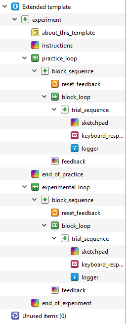
You can permanently delete about_this_template as it just describes the layout of the extended template. You can also permanently delete end_of_practice as we don’t need two messages for this. Start off by changing the name of the experiment by clicking on Extended template in the overview, and changing the name to Eriksen Flanker task by clicking on Extended template in blue. We then want to change the text size to 32, and enter your monitor’s resolution.

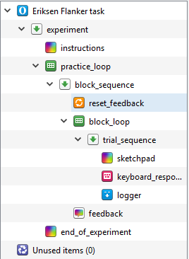
When we made the Stroop task, we only included one block of trials as it was intended to provide a short introduction to creating an experiment using OpenSesame. However, when you create a real experiment, it is a good idea to create a practice block to ensure the participant fully understands what they are doing. One of the helpful features in OpenSesame is the ability to copy and paste a linked component. This means that they are joined, and if you change one of the components, both of them change. This can save a lot of time if the same components are being used with the same settings. In the extended template, the two outer loops (practice_loop and experimental_loop) are independent, but all the components inside them are linked. When you provide people with practice trials, they are usually much shorter than the real experiment as is the case with the design of Rass et al. (2012). Therefore, we are going to delete experimental_loop and edit practice_loop. When we have finished editing practice_loop, we will copy and paste an unlinked version to create another experimental_loop. Right click to delete experimental_loop, and make sure you select permanently delete. If you just click delete, the components will be available in Unused items and it will mess up naming them later. Your Overview should now look like this:

Editing the fixation dot

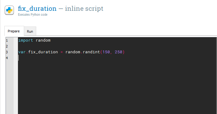
In trial_sequence, there is helpfully a sketchpad component that already includes a fixation dot called sketchpad. Rename this component to fixation. In the trial diagram, fixation is displayed for a random interval between 150ms and 250ms. In the Stroop task, we just set a static duration for 500ms. To create a variable duration, we will need to use our first bit of real Python code. Drag an inline_script component into trial_sequence and place it before fixation. This component allows you to write Python code that can be used in your experiment. Rename it fix_duration as it will control how long our fixation dot is presented for. Within an inline script component, there are two tabs: Prepare and Run. The difference is not important here as we will only be creating a random number. However, if you were to create some complicated stimuli, it can take longer to prepare which affects the timing of the experiment. Therefore, it is better to prepare the stimuli in advance using the Prepare tab, and these can then be presented when necessary using the Run tab. For this example, we will just be writing two lines of code in the Prepare tab. On the first line, type:

import random

It is very important these are all lowercase as Python code is case sensitive. This imports a library called random. A library is a collection of Python code which have specific functions. Random has different functions for creating random numbers. On a new line (it does not matter whether it is on line 2 or 3), we need to create a new variable called fix_duration using the following code:

var.fix_duration = random.randint(150, 250)

This should look like the following:

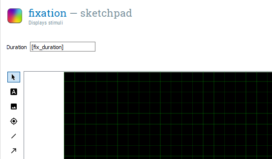
We will take some time to unpack what this is doing. The first part var.fix_duration is creating a new variable called fix_duration. OpenSesame uses the var object to access and create experimental variables in inline scripts. We use the equals sign to assign fix_duration with a number created by the second part of the code. The second part random.randint(150, 250) is accessing a function within the random library called randint. This creates a random integer (whole number) between two numbers which you specify. As we want a random duration between 150ms and 250ms, we enter 150 and 250. Therefore, at the start of every trial (as we put fix_duration within block_loop), we get a new random value for fix_duration. For example, on the first trial it could be 250, on the second 178, and so on. This discourages the participant from mindlessly responding in a predictable fashion. As we created a new variable, we can use this to determine the Duration of fixation using square brackets. If you type [fix_duration] in the Duration of fixation, you should have a component that looks like this:

Creating a stimulus component

Drag a new sketchpad component called stimulus and place it after fixation. Create a text element in the centre of the stimulus screen at coordinates 0,0 and type ‘[stimulus]’. We have not created a stimulus variable in block_loop yet, but we are preempting doing it later. From the trial diagram, we need to change the Duration to 80ms. This displays the stimuli very briefly.

Creating a blank response screen and keyboard response

For the participant to provide a response, we need two components. We need a blank sketchpad component which we can call response_screen and place after stimulus. Set the Duration to 0 as we want the time allowed to be controlled by keyboard_response which was helpfully already present from the extended template.

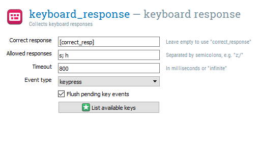
We can edit keyboard_response for this task. In Correct response, we can preempt creating a variable by typing ‘[correct_resp]’. We only need two responses, so type ‘s; h’ in Allowed responses. We want the participant to respond within 800ms, so set Timeout to 800. This means that if the participant takes longer than 800ms to respond, the response is classified as None and incorrect. The keyboard_response component should look like this now:

Creating another blank screen

Now we need another blank sketchpad component called blank_screen that has a duration of 300ms. This should be placed after keyboard_response. At this point in the trial, the participant is provided with feedback on whether they pressed the correct button or not.

Creating feedback screens

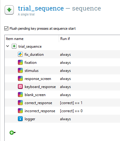
We need two more sketchpad components placed in the centre of both screens called correct_response and incorrect_response placed after blank_screen. Both components should have a Duration of 500ms. We need a text element placed in the centre of both screens. In correct_response, we need a ‘+’ to denote a correct response, and in incorrect_response we need a ‘-’ to denote an incorrect response. If we left the components like this, OpenSesame would display one and then the other. We need to use a bit of Python trickery to control which component is displayed depending on the response. If you click on trial_sequence, you will see a list of all the components within it. There is a second column called Run if. By default, this is set to always, so each component is displayed on every trial. We can modify this and use the correct variable that is updated on every trial. So if the participant pressed the correct button, this would be recorded as a 1, and if they pressed the wrong button, this would be recorded as a 0. Where it says always, change it to [correct] == 1 next to correct_response, and [correct] == 0 next to incorrect_response. The square brackets means we want to access a variable, and 1 and 0 refers to a correct or incorrect response. The two equals signs compares the values either side of the ==. If they match, it is evaluated as true, and if they do not, it is evaluated as false. Therefore, when we have a correct response, correct_response is run, and when we have an incorrect response, incorrect_response is run. At this point, trial_sequence should look like this:

Creating one final blank screen

The final component we need here is a final blank screen which Rass et al. (2012) call the inter-stimulus interval. Drag and place a new sketchpad component called isi after incorrect_response and set the Duration to 500ms. The logger component is already in place from the extended template, so we just need to add some variables in block_loop before we can test if the experiment works at this point.

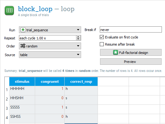
Creating variables in block_loop

In block_loop, we need three columns: stimulus, congruent, and correct_resp. These need to be typed exactly as they were in the components from earlier. The stimulus variable should have four rows: HHHHH, HHSHH, SSSSS, and SSHSS. This covers all the stimuli outlined in the trial diagram. The congruent variable should be a 1 if the letters are all the same, and a 0 if the outer letters are different to the middle letter. Finally, correct_resp should be h or s depending on whether the middle letter is a h or s. The block_loop should now look like this:

Time to test the task

Now is the time to test out the task using quick run . It should run through all of the components and present four trials. We do not need to modify the instruction components yet as it is only to make sure the trials are presenting as they should do. If you have copied all the instructions exactly, it should work. If you get an error message, try and track down the problem. If it crashes, it will try and provide you with instructions on where the error was. Look for any typos or if you forgot to follow any of the steps.

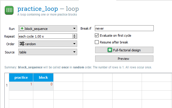
Editing practice_loop

Before we duplicate practice_loop to create a set of experimental trials, we will adapt the loop settings to create some variables for the data file. In practice_loop, there is already one variable and row called practice and yes. We will change this slightly to say 1 instead of yes. Remember we usually use 1 to mean true. Practice trials are not included when you process the data, so this will make it easy to exclude them later on. We will then add a new variable called block with one row and a 0. We are using a 0 as we will be labelling each experimental block as 1-4. The practice_loop component should now look like this:

Creating an experimental loop

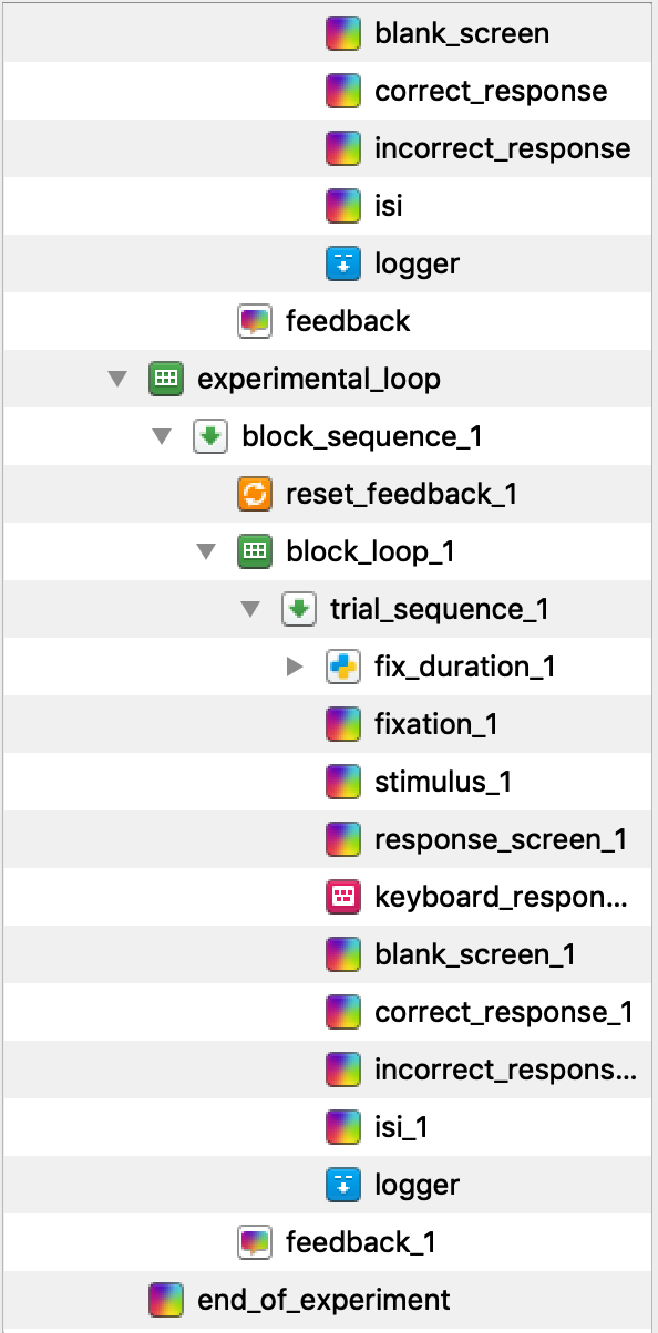
Now is the time to copy and paste practice_loop to create our experimental loop. It is very important that we copy an unlinked version of the component, as we want to add some components without changing practice_loop. As you cannot have duplicate component names, all of the new components will have _1 appended to their names. Change the name of practice_loop_1 to experimental_loop. We also do not want two unlinked logger components. This will effectively cause the data file to be twice as wide as each variable is recorded twice. Permanently delete logger_1 and copy and paste a linked version of logger in its place. You should now have an Overview that looks like this at the bottom (note this is missing some of the components at the top):

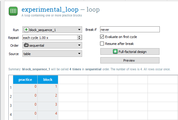
Editing experimental_loop

We will start by creating some variables in experimental_loop. Instead of block reading 0, we now want four rows with the numbers 1 to 4. This is because we will have four experimental blocks. You can then change the practice variable to have a 0 in each of the four rows as they are no longer practice blocks. Finally, change the Order to sequential so the data file is always organised as blocks 1 to 4. This will come in handy later when we will use the block variable to control when a break screen is displayed. The experimental_loop component should now look like this:

Creating a break for participants

After the end of each experimental block, we want to provide the participant with a break. As the final version of the task has 100 trials in each block, it can be mentally draining, so it is a good idea to provide your participants with an opportunity to rest their eyes. We will change feedback_1 to tell them they have 30 seconds to rest. Double click on the existing text when it changes to a grey colour, and write another line to read ‘You now have a 30 second break.’. By default, the font size is 18. Click on the settings icon in the top right corner and click on view script. Change the font size to 32 instead of 18 and click apply and close. We will have to do this for each sketchpad component we edit as changing the default font size only applies to new text elements. Change the Duration to 30000 as this will display the screen for 30 seconds.

Telling the participants when their break is over

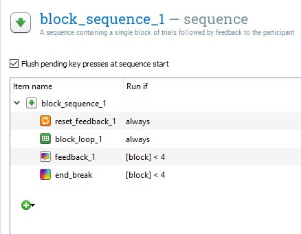
We then want to create a new sketchpad component called end_break and place it after feedback_1 within block_sequence_1. In this component, we just need a text element informing the participant their break has finished and to press any key to start the next block. Duration is set to keypress by default so you do not have to change this. This is to ensure the participant can begin when they are ready.

Controlling when the breaks are presented

If we left it like this, feedback_1 and end_break would run at the end of every block, even at the end of the experiment. This is not necessary, so we can edit the Run if settings in block_sequence_1 to prevent this. Change always to [block] < 4 for both feedback_1 and end_break. This means that these two components will only run on blocks 1 to 3. After the fourth block, we will just get the end of experiment message which tidies the task up. The block_sequence_1 component should now look like this:

Test that the task works again

This is the next point where we should make sure the task is working as intended. Use quick run to test it is working with only 4 trials in each block. It is a good idea to keep the number of trials very small at the testing stage, so that if there is a mistake later in the experiment that causes it to crash, you have not spent 10 minutes working through the task. If you followed all the instructions, the task should run and there should only be three breaks.

Increasing the number of trials

At this point, the skeleton of the task is complete and working as we want it to. All we have left to do is edit all of the messages to be informative and increase the number of trials. Make sure you edit instructions, feedback, and end_of_experiment. Make sure the participants are informed in feedback they will be starting the main experimental trials when they press a button. We know from the instructions in Rass et al. (2012) that there were 20 practice trials and 100 trials in each experimental block. In block_loop, change the repeat setting to 5 to create 20 trials. In block_loop_1, change the repeat setting to 25 to create 100 trials. You can now run the task full screen to test it out and get a full data set to explore in the next section.

Analysing response time data from the Eriksen Flanker task

After running the task, you should have a data set with 420 trials to work with. Follow the same instructions as task one to import the data set into SPSS as a .csv file depending on whether you are using version 23 or 25 of SPSS. Before looking at the reaction times, we will follow the same procedure as task one and remove any extreme and incorrect responses.

Removing unwanted trials

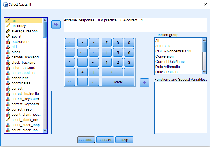
Follow the previous instructions from task one to code extreme responses as 1 and acceptable responses as 0. For this experiment, we will also remove the practice trials. If you click on Data > Select Cases, and then if condition is satisfied, we need to specify three criteria: correct = 1 & practice = 0 & extreme_response = 0. Your window should look like this:

If you click Continue and then OK, SPSS will remove the first 20 rows and any incorrect/extreme responses. You will probably notice that you made quite a few errors. The aim of this task in Rass et al. (2012) was to force participants to make several mistakes as they were interested in how participants responded to making errors using EEG. My accuracy was approximately 85% in each block.

Calculating the response time to congruent and incongruent trials

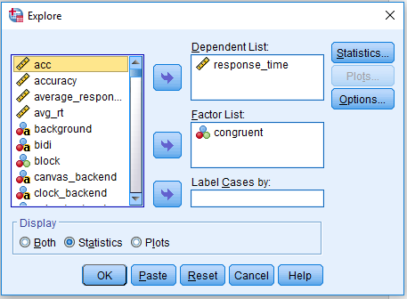
We can now look at the difference in respone time between congruent and incongruent trials. In order to calculate the median response time, click Analyze > Descriptive Statistics > Explore. Drag response_time into Dependent List and congruent into Factor List. Select Statistics under Display, and click OK to get the output. The Explore window should look like this:

For my data, my median reaction time to congruent stimuli (congruent = 1) was 330ms, but for incongruent stimuli (congruent = 0) it was 363ms. This shows a small effect of distracting noise on target identification. If you were to run an experiment using this task, you would record these values per participant like this:

participant	congruent_rt	incongruent_rt
1	330	363

Exercises

Excercise 1. Reuse trial sequence in the flanker task

Don’t Repeat Yourself (DRY) is a principle of software development. Why? One main reason is that it helps to avoid redunancy in your code. Moreover, if you change information at one place and forget to do it another place this mistake will be very hard to detect and may get unnoticed for any future users too. Let’s improve the experiment you created during the flanker task tutorial during the last session by applying this principle.

At the moment we do repeat ourselves by using a copy of the trial_sequence of the practice block in the test block. Moreover, all objects within the trial_sequence_1(except the logger) are copies too! This is not necessary because the trials in the practice block and the test block are identical. So block_loop_1 can simply run the same sequence as block_loop. So, permanently remove trial_sequence_1 and all the copied objects within it. Then, change the block_loop_1 and let it run trial_sequence instead.

Excercise 2. Change the number of trials in the flanker task

Brysbaert and Stevens (2018) have suggested that you need at least 1,600 observations per condition to observe RT effects of around 15 ms in a within-subject design. Assume for a moment that the flanker congruency effect is that small (typically it is larger) and you want to run 10 participants in your study. How many observations do you need for each subject and each congruency level? Use the corresponding number to adapt the number of trials presented in the flanker task you just created.

References

Brysbaert, M., & Stevens, M. (2018). Power analysis and effect size in mixed effects models: A tutorial. Journal of cognition, 1(1).

Detandt, S., Bazan, A., Schröder, E., Olyff, G., Kajosch, H., Verbanck, P., & Campanella, S. (2017). A smoking-related background helps moderate smokers to focus: An event-related potential study using a Go-NoGo task. Clinical Neurophysiology, 128(10), 1872–1885

Mathôt, S., Schreij, D., & Theeuwes, J. (2012). OpenSesame: An open-source, graphical experiment builder for the social sciences. Behavior research methods, 44(2), 314-324

Lachaud, C. M., & Renaud, O. (2011). A tutorial for analyzing human reaction times: How to filter data, manage missing values, and choose a statistical model. Applied Psycholinguistics, 32(2), 389-416.

Leys, C., Ley, C., Klein, O., Bernard, P., & Licata, L. (2013). Detecting outliers: Do not use standard deviation around the mean, use absolute deviation around the median. Journal of Experimental Social Psychology, 49(3), 764–766.

Peirce, J. and MacAskill, M. (2018). Building Experiments in PsychoPy. London: SAGE.

Petit, G., Kornreich, C., Noël, X., Verbanck, P., & Campanella, S. (2012). Alcohol-related context modulates performance of social drinkers in a visual Go/No-Go task: a preliminary assessment of event-related potentials. PloS one, 7(5), e37466

Rass, O., Fridberg, D. J., & O’Donnell, B. F. (2014). Neural correlates of performance monitoring in daily and intermittent smokers. Clinical Neurophysiology, 125(7), 1417–1426

Ratcliff, R. (1993). Methods for Dealing With Reaction Time Outliers. Psychological Bulletin, 114(3), 510–532.

Wessel, J. R. (2018). Prepotent motor activity and inhibitory control demands in different variants of the go/no-go paradigm. Psychophysiology, 55(3), 1–14