Go-nogo task in OpenSesame

Go-nogo task in OpenSesame#

Note: The text below is adapted from the OpenSesame guide by James E. Bartlett licensed under CC-By Attribution 4.0 International.

Tutorial 3. Go-NoGo task with images#

In this tutorial we are going to create another commonly used cognitive task known as the Go-NoGo task. This measures inhibitory control, or the ability to stop a behaviour once you have started to make it. The standard version of the task presents a series of Go stimuli on the screen, for example a green circle or the letter ‘x’. Every time the participants sees the circle or letter they have to press a button on a keyboard. However, on a small number of trials (20% or fewer), a NoGo stimulus is presented, for example a red circle or the letter ‘o’. This time, they have to avoid pressing the button. Because of how fast the trials progress and the infrequency of the NoGo stimuli, it can be difficult to inhibit the response. The version of the task we are going to recreate is adapted to incorporate different types of images and is based on the task used in Dedandt et al. (2017). This will show you how you can incorporate images into your OpenSesame task.

Recreating the Go-NoGo task#

Dedandt et al. (2017) were interested in comparing smokers and non-smokers on their ability to inhibit a response. They were also interested if different backgrounds would influence the smokers’ ability to inhibit a response. Therefore, three different backgrounds were used: a smoking cue, a non-smoking cue, and a neutral cue. If we look in the method section of Dedandt et al. (2017), there is a task diagram and a description of the task. We will go through the design of each trial, and how the whole task is structured.

What is the structure of one trial?#

For the structure of each trial, the authors include this helpful diagram on page 1876 (this is cropped slightly):

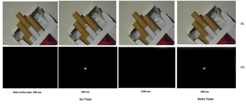
We can see from the diagram that each trial begins with the presentation of the background for 500ms. In contrast to our two previous tasks, there does not appear to be a fixation cross/dot included in this task. A Go or NoGo cue is then presented on the screen for 200ms. On Go trials, this is a letter ‘M’ superimposed onto the background. On NoGo trials, this is the letter ‘W’. After the offset of the cue, there is a 1300ms period where the participant can make a response. The start of the next trial then begins with the next 500ms screen.

What is the structure of the whole experiment?#

For the structure of the whole task, the study explains there are six experimental blocks. There were five backgrounds used in the task, two smoking images, two non-smoking images, and a blank black background. In contrast to Rass et al. (2012) in the last section, there is quite a bit of missing information that we would need to fully reproduce the task. First, there is no mention of a practice block. Second, the study does not explain that the same black background is used in two blocks. Third, it is not directly explained that one background is shown per block. You can work it out from the introduction and other information in the methods section, but it is not directly specified. These details can be found in another paper which the methodology is based on (Petit et al. 2012). This is a common occurrence, as research teams often produce several publications based on the same method, but to prevent repeating the details in each article, they just reference the first. Finally, it does not explain what kind of break was provided to the participants in between each block. We will give people 30 seconds in order to rest their eyes.

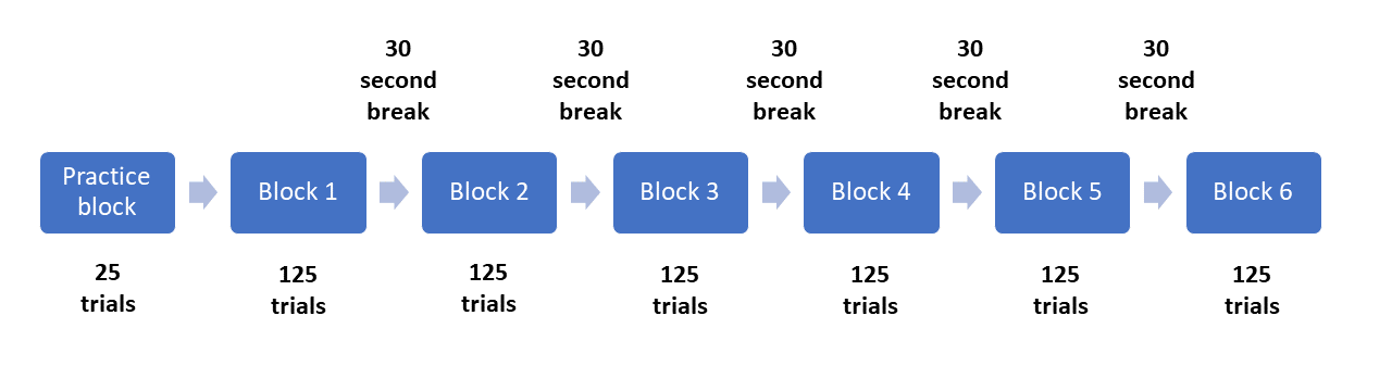
Although we are trying to recreate the task from Dedandt et al. (2017), there is one feature we are going to consciously change: the proportion of Go and NoGo trials. In order to measure inhibitory control, the response to Go stimuli should be be prepotent, meaning you should want to quickly respond, in comparison to the NoGo trials. A long list of studies have been criticised for having too many NoGo trials (Wessel 2017; for a graphical explanation, see FlexibleMeasures). Therefore, Go-NoGo tasks should have a maximum of 20% NoGo trials. As Dedandt et al. (2017) had 30% of the trials as NoGo, we are going to tweak it slightly to be a more valid measure of inhibitory control. Therefore, instead of including 93 Go and 40 NoGo trials per block, we will include 100 Go trials and 25 NoGo trials per block. Similar to the Eriksen Flanker task, we can visualise the structure of the whole experiment like this:

Creating the task in OpenSesame#

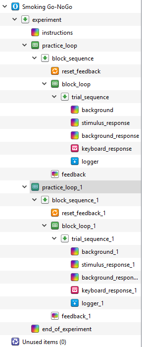
To start this task, we will use the extended template to create the general structure of the experiment. Click on Extended template in the Overview window. Begin by changing the title of the experiment to “Smoking Go-NoGo” by clicking on the blue main title. The resolution will need changing to your monitor’s dimensions, and the default text size should be 32 px. Permanently delete the experimental_loop so we can change the number of trials later without having to change all the blocks.

Adding images to the file pool#

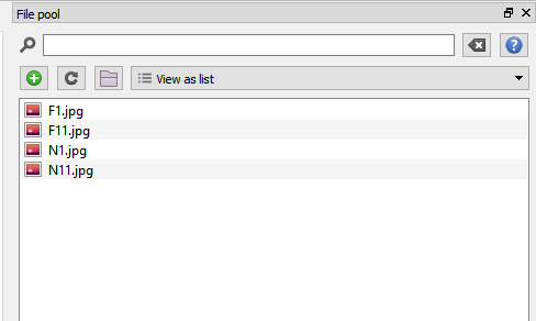
This task will use images (these can be downloaded here) as the background in order to manipulate the type of cues the participant is viewing. If we want to use images in OpenSesame, we need to make them accessible. To do this, we need to add them to the file pool , and click the small green add symbol. This will allow you to browse your computer and select the files. When you have added all four images, the file pool should look like this:

Creating the background screen#

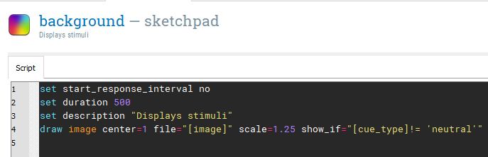
We will create a single trial in trial_sequence using three different components. The first component will be a blank background and we can rename sketchpad to background. The start of each trial is just the background which is presented for 500ms. For each block, the background will be an image we added to the file pool or a plain black screen. This means we need to insert an image element into the centre of the screen at coordinate 0,0. When you click where you want the image, you will be prompted to select an image from the file pool. Select any image as we will be changing it to a variable later.

We need to adapt the script, so click on View script under settings

Creating the response screen#

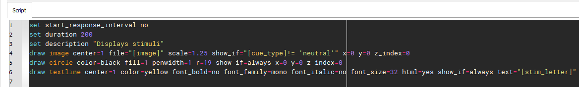
The next component we need is to display the cue that participants will need to respond to. To save having to repeat the procedure for the last component, copy and paste an unlinked version of background after the first background, and rename it stimulus_response. This component should have a duration of 200ms. This will be the same screen, but with a response cue and black circle superimposed on the background image. First, select a circle element and make the necessary edits. The image element should look the same as in the previous step. The next element is the circle element. In the figure from Dedandt et al. (2017), we can see the circle is solid black. By default, the color of the circle is set to white and not filled (indicated by fill = 0). Change color to black, and fill to 1. Change the radius (r) to 19 as this just covers the size of the text. Now we need to edit the text element. Change color to yellow to be consistent with the original study, and change the text to [stim_letter]. This is short for stimulus letter and we are preempting another variable we will set in the loop. The script for stimulus_response should now look like this:

The final thing to note here is the order of the elements is very important. OpenSesame presents them in layers, so the first element is created first, then the second, and so forth. We need to create the image, then the circle, and then the text. If we had a different order, the text or circle would not be visible, which we do not want. Click apply and close, and we will move on to the next component.

Creating a response screen#

The final sketchpad component we need here is a plain background again, as the stimulus is only presented for 200ms and then disappears. Copy and paste another unlinked version of background after stimulus_response. Change the name to background_response and set the duration to 0. We will be using keyboard_response to control the duration. In keyboard_response, change Correct response to [correct_resp], Allowed responses to ‘m’ as this is the only response we will need, and Timeout to 1300. The logger is already there, so these are all the components we need. We can now start to add in all the variables we have preempted into block_loop.

Defining variables in block_loop#

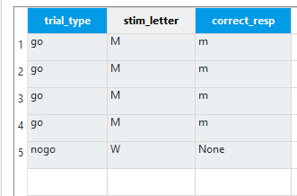
There are three variables we need to change on a trial by trial basis. The first variable we want to define is not relevant for the experiment, but it will be helpful for data analysis later. Label the first variable trial_type and enter four rows of ‘go’ and one row of ‘nogo’. In the second column, type stim_letter to control which letter we are presenting. For each ‘go’ trial enter a capital ‘M’, and for the ‘nogo’ trial enter a capital ‘W’. Finally, create a third variable called correct_resp. For each ‘M’ in stim_letter, write a lowercase ‘m’. For the ‘nogo’ trial where we have a ‘W’, write ‘None’. As we are testing the participant’s ability to resist making a response on ‘nogo’ trials, the correct response should be nothing at all. This means we want keyboard_response to time out, which OpenSesame records for the response as ‘None’. Therefore, if we enter ‘None’ for correct_resp, we will get an accurate recording for correct responses and accuracy in the data file. These are all the variables we need to define in this loop component. The loop should look like this when you have finished:

Defining the background image in practice_loop#

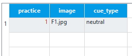
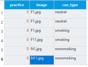
At this point, you may be thinking where we will define the background image. We saw from Dedandt et al. (2017) that we want one image to be presented per block in order to display the same background for a long period of time. Therefore, we are going to define the background image in the outer loop called practice_loop. As this is the practice loop, we only want one block to let the participant try out the task and make sure they understand what they’re doing. The first variable should be practice, and this should be set to 1 to indicate true. The second variable should be ‘image’ and set to ‘F1.jpg’ in reference to one of the images we saved in the file pool. Finally, we need a variable called ‘cue_type’ with one row set to ‘neutral’. During the practice block, it is best to avoid using stimuli that will be in the experimental blocks as the participants may get used to it. We are only defining this image here as we need the image to exist in our file pool or the experiment will crash. However, as we are setting cue_type to ‘neutral’, the image will not display because of how we defined the show_if argument in the image elements. For the practice block, we will just present the participants with a blank black screen. The practice_loop component should now look like this:

Test the experiment#

At this point, we can test the experiment to make sure it works in its current form. If everything has been defined correctly, you should be able to quick run the experiment and complete five trials. Remember you should avoid making a response when the letter ‘W’ appears.

Creating the experimental_loop#

Now that we know the task works in principle, we can scale it up to include experimental blocks and change the background image. Copy and paste an unlinked version of practice_loop and place it after end_of_practice. We do not need end_of_practice, so you can permanently delete it. The overview of your experiment should now look like this:

Rename practice_loop_1 to experimental_loop, and permanently delete logger_1. Copy and paste a linked version of logger in the place of logger_1 after keyboard_response_1. This will ensure we have a tidier data file.

Specifying the background images#

We can now edit experimental_loop to control the background image on each block. The first row should already be there from copying and pasting the loop. This can stay the same as we need one black background screen. All you need to change is practice to 0 as this is now the experimental loop. We will create five more blocks. The image column should have five more rows with F1.jpg, F1.jpg, F11.jpg, N1.jpg, and N11.jpg. For the first two instances of F1.jpg, cue_type should be ‘neutral’ to create two blocks with a black background. For the remaining images starting with ‘F’, cue_type should be ‘smoking’, and for the images starting with ‘N’, cue_type should be ‘nonsmoking’. All the rows should have a 0 for practice. The experimental_loop component should now look like this:

Order should be kept as random, as we want a new order of experimental blocks per participant. At this point, we can test the experiment again using quickrun in order to be certain that all the images are displaying properly and the blocks are presenting as we want them to. One image should be presented in each block, apart from two blocks will just have a black background.

Editing the instruction components#

Now we can focus on tidying up the instructions. The first thing to change is instructions. Here you can edit the text and explain to prospective participants that they need to press the letter ‘m’ when they see an ‘M’, and withhold a response when they see a ‘W’. Remember for any text you are editing, you will need to change the font size to 32 manually by editing the script. In feedback, we need to explain to the participants that they will begin the experimental trials when they press a button. In feedback_1, we need to explain to the participants that they have a 30 second break. Make sure you change the duration to 30000. We now need to insert a new sketchpad component called end_of_break after feedback_1. Write a message explaining to participants that their break has finished and ensure they can start the next block with a keypress. Finally, change end_of_experiment to thank the participants for their time and they can exit the experiment by pressing any button.

Controlling when the breaks are presented#

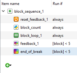
In the last experiment, we stopped feedback_1 and end_of_break from appearing after the final block. Each block was identical, so we just presented each block sequentially and used the number of the fourth block to stop the two components from appearing. However, this time it is not so simple. We cannot simply label each block 1 to 5 as they are being randomly presented. What we need is to label each block as we go along so the background is free to be randomly presented. We can do this by inserting two inline script components called block_count between reset_feedback_1 and block_loop_1 in experimental_loop. Here we need to write var.block = var.block + 1 in the prepare tab. For each loop around experimental_loop this assigns var.block to equal the previous value for block plus one. The positioning of these two inline script components is very important. We want block_start to be outside of experimental_loop as we do not want it to be reset to 0 on on each cycle around the loop. We also want block_count to be in experimental_group and not block_loop_1. If we placed it in block_loop_1, it would increase by one on each trial. We want it to increase by one on each block, so by the time we get to the fifth block, block will equal 5. This means that we can enter some short Python code into block_sequence_1 to control when feedback_1 and end_of_break are run. Where it says always, change it to [block] < 5 for feedback_1 and end_of_break. The block_sequence_1 component should now look like this:

Test the experiment one last time before we increase the number of trials. Use quickrun to test the experiment in a separate screen. The two break screens should not appear after the final break.

Increase the number of trials#

In block_loop, change the number of repeats to 5 to create a practice block featuring 25 trials. In block_loop_1, we need to set the number of repeats to 25 in order to create 125 trials per experimental block. The experiment should now be in its completed form providing all the instruction components have been edited to be informative to the participants.

Test the experiment full screen#

You can now run the experiment full screen to get a data set ready to analyse in the next section. At 750 trials, this is a pretty hefty task so it will take approximately 20-30 minutes to complete.

Analysing the data from the task#

The Go NoGo task provides you with a few options for what you can use as your outcome variable. In the original study by Dedandt et al. (2017), they report three different outcomes: reaction times on Go trials, omission error rates (not pressing a button on Go trials), and commission error rates (pressing a button on Nogo trials). We will go through how you can calculate each one. However, if you were to use this task yourself, it is important to think about which measures you are interested in. Try and avoid analysing several outcomes and seeing which one works unless you are specifically conducting exploratory research.

Import the csv data into SPSS#

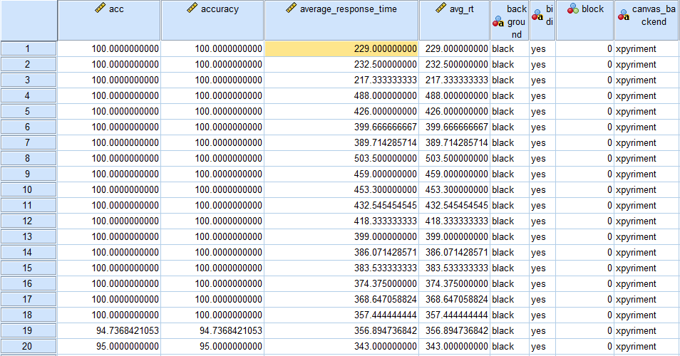
Follow the instructions from the first task for importing the .csv data file from the experiment. You should have a screen that looks like this with 775 rows including the practice trials:

Coding extreme responses#

This time we do not need to take out the incorrect responses as they are important for calculating the error rates. However, we still need to remove the 25 practice trials and extreme responses. Because of the nogo trials, we need to think more carefully about how we exclude extreme responses. In the previous tasks, we excluded any response outside of 100-1000ms. However, on nogo trials, the participants should not be pressing anything, which means the response time should always be 1300ms. This would mean all nogo trials would be excluded if we performed the same extreme response removal procedure. Click on Transform > Recode into Different Variables. We can still call the Output Variable “extreme_response” and create the same Old and New Values. As a reminder, the menus should look like this:

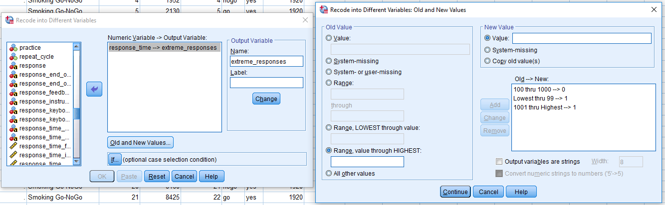
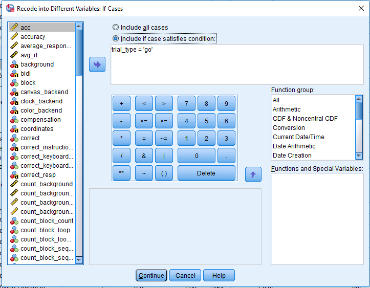
Click Continue on the Old and New Values screen. In the Recode into Different Variables menu, click on If… above the OK button. Click Include if case satisfies condition and type trial_type = ‘go’. This means we only want to recode go trials, and ignore nogo trials for now. The menu should look like this:

Click Continue and OK, and the extreme_response column should have a 1.00 for extreme go responses, 0 for acceptable, and blank for nogo trials. The blank responses are created as we told SPSS to just recode go responses. Blank entries are not helpful, so we need to fill them in with a 0 for nogo trials.

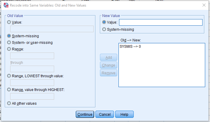
Click Transform > Recode into Same Variables. This allows us to change values in the same column, rather than computing another one as we have done previously. Drag extreme_response into Numeric Variables and click on Old and New Values. Click System-missing under Old Value and type 0 into Value under New Value and click Add. The screen should look like this:

If you click Continue and OK, this will fill in all the missing values with a 0 for our nogo trials.

Removing extreme responses and practice trials#

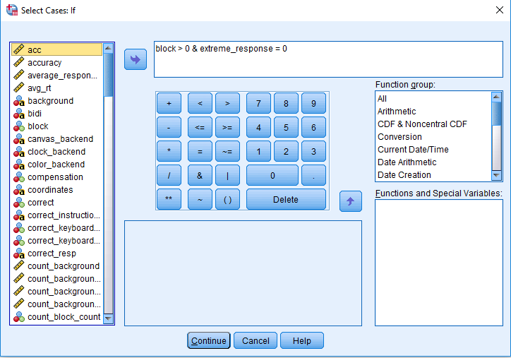
We can now select cases using this the extreme_response column. Click on Data > Select Cases, and if condition is satisfied. As we labelled the blocks starting as 0, we can select block > 0. This will remove the practice block and leave blocks 1-6. In addition, include extreme_response = 0. The select cases window should look like this:

Click continue and OK to apply the select cases. This will cross out any practice trials and extreme go responses. Remember we want to retain incorrect responses for the analysis of error rates.

Calculating error rates#

We can calculate the omission and commission error rates together. Click on Analyze > Descriptive Statistics > Explore. Drag the correct variable In the Dependent List box. One of the benefits of coding correct and incorrect responses as 1 and 0 is calculating the mean provides you with the percentage correct. For example, if you have 100 trials and get 75 correct, the mean of the correct variable would be 0.75 (75%). Now drag cue_type and trial_type into Factor List. Finally, we only need statistics so click Statistics under display. If we pressed OK now, we would get two outputs, one table for correct split by cue_type, and one table for correct split by trial_type. SPSS can be stubborn and does not provide us with the option to split correct by the combination of cue_type and trial_type through the menu. However, we can edit the underlying syntax to get SPSS to do it. Click on Paste and this is the underlying syntax that SPSS uses to specify the analyses. You should have a window that looks like this:

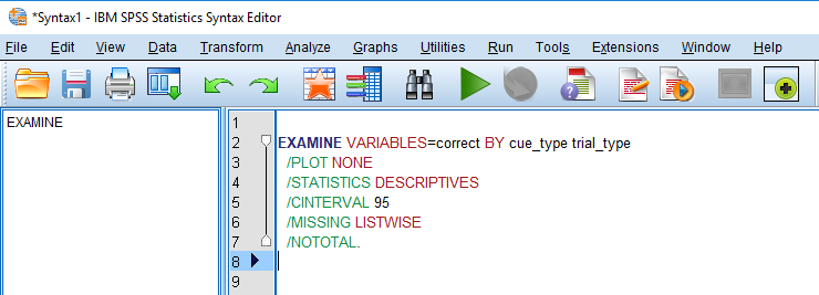We are interested in the first line of syntax. This is telling us we are examining correct by cue_type and trial_type. In order to examine correct by the interaction of the two variables, we simply need to add a star (*) between the two factors. This tells SPSS we want the combination of the two variables. You should now have a syntax screen that looks like this:

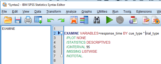
In order to get the statistics, we need to click the big green arrow to run the syntax. In the SPSS output, the first table should look like this:

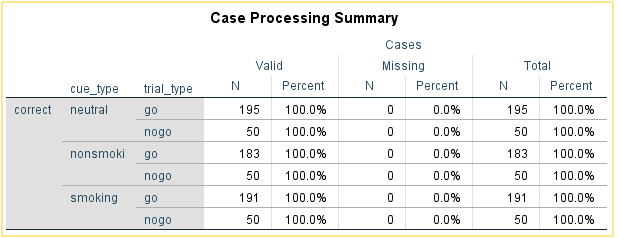This tells us we should have the information we want and correct is broken down by the combination of cue_type and trial_type. Note there are some missing go trials because of extreme responses. In order to get our first two outcome variables, we need the mean of correct for each combination of the variables in the Descriptives table. The Descriptives table should look like this:

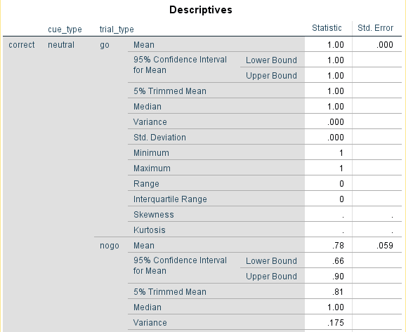
This is a shortened version that shows the output for the neutral cue_type. In order to get the same outcome variable as Dedandt et al. (2017), we need to subtract the mean from 1 for both go and nogo trials. For my data, I would record the different conditions like this in my data file:

Participant	neutral_go	neutral_nogo	smoking_go	smoking_nogo	nonsmoking_go	nonsmoking_nogo
1	0	0.22	0	0.20	0	0.22

This shows that I did not make any omission errors, and my commision error rate was around 20% for each cue condition.

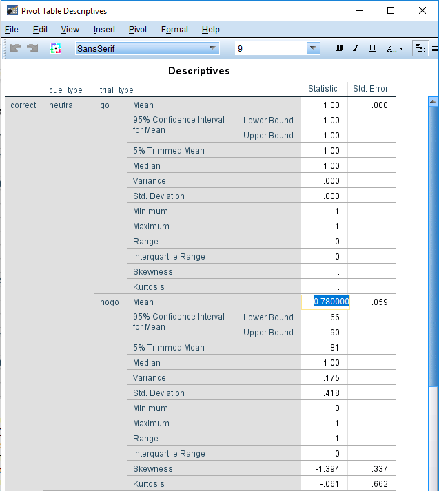
Reporting greater precision#

SPSS usually reports to two decimal places, which is fine for most purposes, and it is the precision reported in the original article. However, if we wanted a more precise answer, you can see the full number by double clicking on the table and clicking on the cell you are interested in. It should look like this:

Calculating the response time to go stimuli#

Calculating the median RT follows the same process as before but using response_time as the dependent variable instead of correct. This time we do have to remove incorrect responses as they may be an unreliable source for the response times. Edit the Select Cases menu and add correct = 1. It should now read: block > 0 & extreme_response = 0 & correct = 1. In order to calculate the median RT, follow the instructions from the last example for the explore menu but replace correct with response_time. When you click paste and add the * between the two factors, the syntax window should now look like this:

All that we replaced is response_time before BY cue_type * trial_type. We could have even wrote this in the syntax ourselves if we typed it exactly as it is in the data file. Press the green arrow to run the syntax again. For the descriptives table in the output, you should have something that looks like this:

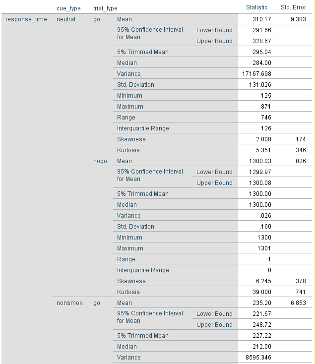
We are only interested in the go trials this time, so we only need to record three values. For my data I would record it like this:

participant	neutral_rt	smoking_rt	non-smoking_rt
1	284	213	212

Tips for Debugging Experiments#

Debugging an experiment requires problem solving and can be considered a skill in itself. It is similar to the process of science. You have a hypothesis about a problem you are facing. You systematically test the sources of the problem until you isolate it, and then fix the problem. Most of this guide is based on using the OpenSesame GUI, and you will generally encounter fewer bugs than if you were to write your experiment using scripts. However, you will still encounter problems with implementing your ideas. Perhaps your images are not presenting how you want them to, or your feedback is not working. Solving these problems is very similar to solving problems in code. Some of this advice is taken from the excellent book on another Python based experiment builder called PsychoPy (Peirce and MacAskill, 2018).

Steps to take when debugging#

Read the error messages carefully. If your experiment crashes, OpenSesame does its very best to tell you what caused the problem. Take task three as an example. I run the experiment, and as soon as I press a key after the instructions, the experiment closes and I get the following message:

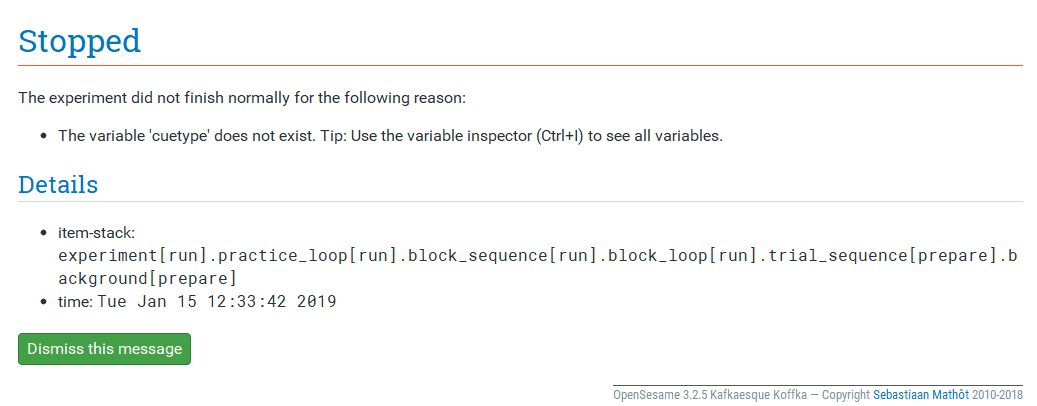
OpenSesame provides us with a reason for the experiment crashing: thevariable “cuetype” does not exist. At this point, you realise youmissed the underscore and it should be “cue_type”. Not all of theproblems will be this easy, but you should be directed by OpenSesameto the simple fixes.

Look for typos carefully. In my own experience, a stray typo is one of the most common causes of an experiment crashing. As Python is case sensitive, it can be difficult to spot the difference between image and Image. Likewise, the difference between colour and color may be hard to spot. If you are struggling to find typos, you may just be too tired. Make sure you take frequent breaks to prevent being fatigued.
Test your experiments in a separate window. When testing your experiments, always run it in a separate window until you know it works. If you run your experiment full-screen, you may have made a mistake that causes it to freeze and you will be unable to escape it. At best, you just have to restart your computer. At worst, you may have lost an hour’s worth of work if you did not save it beforehand.
Be methodical. If you do not know the source of the problem immediately, change one thing at a time until the experiment works. In an ideal world, get into the habit of testing your experiment after every addition. This means you should know which addition caused the problem in the first place. You can then investigate what it is about that addition that caused the problems.

Asking for help#

The aim of this guide is to provide you with support to create experiments on your own. However, there will be times where you do not know how to put your idea into practice, or you cannot figure out what is wrong with your experiment. If you are asking for help, the person you are asking will not be very happy if you just say “it doesn’t work”. They will be very grateful if you can break it down and say “I have tried these steps, but it does not work”, or “I have narrowed it down to X, but I cannot work out what is wrong with it”. In my experience, the act of writing down the steps you have taken to solve the problem can often lead you to the solution yourself as you see the bigger picture.

Exercises#

Excercise 1. Counterbalancing: Even or odd participant numbers#

Open the Stroop task you created during the earlier tutorial. Adapt the correct response by using the numeric button 1, 2, 3, and 4 of the keyboard.

Combine loops and conditional running (use the experimental variable subject_parity, see https://osdoc.cogsci.nl/manual/variables/) to generate the correct response for the four colors. For even-numbered participant numbers (version 1), use the following mapping:

red > 1

green > 2

blue > 3

yellow > 4

For odd-numbered participant numbers (version 2), use the following mapping:

red > 3

green > 4

blue > 1

yellow > 2

Indicate the correct mapping in the instructions.

Note: do not create two versions of the same experiment, just program the counterbalancing in one file. Do not forget to log the version number. Check whether your solution works properly.

Excercise 2. Show mapping of correct keys on the screen#

Please add four rectangles to the bottom of the stimulus display to remind the participant of the correct order. Ensure that the colors of the correct response are presented in the right order, depending on the version of the experiment.

References#

Brysbaert, M., & Stevens, M. (2018). Power analysis and effect size in mixed effects models: A tutorial. Journal of cognition, 1(1).

Detandt, S., Bazan, A., Schröder, E., Olyff, G., Kajosch, H., Verbanck, P., & Campanella, S. (2017). A smoking-related background helps moderate smokers to focus: An event-related potential study using a Go-NoGo task. Clinical Neurophysiology, 128(10), 1872–1885

Mathôt, S., Schreij, D., & Theeuwes, J. (2012). OpenSesame: An open-source, graphical experiment builder for the social sciences. Behavior research methods, 44(2), 314-324

Lachaud, C. M., & Renaud, O. (2011). A tutorial for analyzing human reaction times: How to filter data, manage missing values, and choose a statistical model. Applied Psycholinguistics, 32(2), 389-416.

Leys, C., Ley, C., Klein, O., Bernard, P., & Licata, L. (2013). Detecting outliers: Do not use standard deviation around the mean, use absolute deviation around the median. Journal of Experimental Social Psychology, 49(3), 764–766.

Peirce, J. and MacAskill, M. (2018). Building Experiments in PsychoPy. London: SAGE.

Petit, G., Kornreich, C., Noël, X., Verbanck, P., & Campanella, S. (2012). Alcohol-related context modulates performance of social drinkers in a visual Go/No-Go task: a preliminary assessment of event-related potentials. PloS one, 7(5), e37466

Rass, O., Fridberg, D. J., & O’Donnell, B. F. (2014). Neural correlates of performance monitoring in daily and intermittent smokers. Clinical Neurophysiology, 125(7), 1417–1426

Ratcliff, R. (1993). Methods for Dealing With Reaction Time Outliers. Psychological Bulletin, 114(3), 510–532.

Wessel, J. R. (2018). Prepotent motor activity and inhibitory control demands in different variants of the go/no-go paradigm. Psychophysiology, 55(3), 1–14